The ever-increasing volume and diversity of data available to an actuary is both exciting and terrifying. Exciting because of the amazing and unexpected findings waiting to be discovered, and terrifying because of the drudgery and disappointment to be endured along the way. Compounding the matter is the shrinking time frames to discover insights and turn them into action.

Just as technology rewards us with a mess of data, technology helps us sift through it. Excel unable to handle tens of millions of rows? Robust data visualization software is a download away. Need to fit statistical models? Statistical packages such as R carry a plethora of tools to illuminate the finest details.

Brief History of Analysis

Actuaries have traditionally analyzed data using manual methods. Even with the assist of technology, an actuary is manually reviewing, evaluating, and judging the fitness of data for its intended purposes. While some details of the analysis will differ depending on the data, the traditional approach often follows a recipe like this one for mortality analysis:

1.  Look through the dimensions of the data to find credible and significant factors driving mortality.

• To start, one dimension is considered at a time.
• Optionally, two or more dimensions can be considered at the same time.
• Filters can be introduced at any point.

2. Develop a set of factors for that dimension or combination of dimensions.

3. Do one of the following:

• Adjust the experience with the new factors.
• Set the factors aside (don’t adjust).

4. Go back to 1 if further adjustments are needed.

5. If nothing needs to be changed, check for reasonableness and fit.

The recipe works, but is not without shortcomings.

1. Sifting through potential factors, including combinations of factors and filters, is labor intensive, and it is probable that some important factors and combinations in a large or complicated dataset will be overlooked.
2. When to stop looking for factors is left to judgment. The risk is that the modeler could either stop too early and miss important factors, or stop too late and waste valuable time.
3. For reasons of expediency or inexperience, factors are sometimes not fit simultaneously. If there are dependencies between factors, the factor estimates may change in the presence of its related factors. For example, perhaps I have derived a factor of 120% for males and 90% for females. I then find smoker status is important, say 190% for smokers and 95% for non-smokers. If there are a lot of smokers in the male category, the factor for males is being overstated in part by the smokers differential.
4. It can happen that different types of models suit different parts of the data. For example, an interaction of dimensions in one section of the data might be unneeded in another.

Dessert Before Dinner

In the fall of 2018, the Society of Actuaries issued a data challenge whereby the Individual Life Experience Committee (ILEC) released experience data from 2009 to 2015 and invited interested parties to compete to submit the best data analysis solution. The top three entrants were awarded fabulous cash prizes.

The dataset contains 30.6 million rows. There are 3,443,319 claims on 352.5 million life year exposed, resulting in $179.4 billion in claims on 71.1 trillion dollar years exposed.

Consider the following findings for term experience:

1. The mortality experience for term business having at most one preferred class (and hence two risk classes) deteriorated significantly over the study period.
2. At the same time, experience for 3- and 4-risk class systems improved significantly.
3. Term experience with face amounts below $100,000 generally deteriorated.

How did I discover this? Is there anything else hiding in the data? And where did the interesting graphic below come from?

GLM Trees

In the early days of my mortality modeling (late 2000s), GLMs and GAMs were the best available tools. Computing power was not yet available for more sophisticated modeling. In some cases, today’s algorithms had not been invented yet or had not yet diffused through the broader statistical and actuarial communities.

Model fitting with GAMs can be a chore. Stepwise feature selection as implemented for GLMs does not work with splines, and once splines are in play, the model building process gets more manual. To ease the burden, I searched the literature for methods for automated feature and interaction detection. One can find a number of approaches, including chi-square automatic interaction detection (CHAID) and other decision tree types. CHAID had many of the features I wanted, yet it appeared to be incompatible with the A/E and qx analyses I was doing.

In 2008, Achim Zeileis, Torsten Hothorn, and Kurt Hornik introduced a rigorous theoretical framework built on decades of research into combining parametric models such as GLMs with decision tree models. The algorithm relies heavily on parameter fluctuation tests. The tests are used to detect whether there is unmodeled variation in the residuals from the regression models.

If you were building a model by hand, you might fit a model and then check how well the model fits the data by examining one or more dimensions. For example, if you fit a constant percentage and then look at fluctuations of actual-to-model mortality in a pivot table, you might note some residual variation for some dimensions but not others. The visual variation may just look like noise, or it might show some trends or regular patterns in the actual-to-model mortality.

In the case of model-based recursive partitioning, that last part about residual variation looking like noise is the start of understanding how variations are detected algorithmically. For an ordered dimension (like age or experience year), under the null hypothesis that the residuals are independent, identically distributed random variables, the running sum of the residuals is asymptotically distributed as a Brownian bridge (that is, a random walk starting and ending at 0), subject to appropriate scaling. In the unordered case (like gender or other categories), a Chi-square goodness-of-fit test is applied to the residuals for that dimension.

The dimension with the most variation across all regression parameters wins. The algorithm then goes about searching for the best binary subdivision for that dimension. For an ordered dimension, each break point in the data is tested sequentially. For an unordered dimension having n levels, the algorithm tries all of the binary subdivisions of the dimensions. There are 2^n-1-1 possible subset breaks to check. In both cases, the partition which maximizes the likelihood the most wins.

Now that the data have been broken into two subsets, the algorithm starts the process over on the smaller pieces. Eventually, the recursive partition procedure stops, either because there is nothing to improve or because the analyst specified a stopping rule.

A Concrete Example

Since mortality trend is among the most important topics for life insurance pricing, I had attempted several model types, including GLMs/GAMs, elastic net regression, boosted trees, and GLM trees. As it happens, only GLM trees were able to discover what subsets of the data had meaningful differences in mortality levels and trends.

To start, I opted to use the Poisson regression model of

Number of Deaths ~ b₀ + b₁ Experience Year
+ log (Expected Claims 2015VBT)

The partitioning variables are everything else. Because some variables are insurance plan specific, I carried out the analysis separately for term and permanent products. This example follows the algorithm and results for the term analysis. Since this is an exploratory exercise, no training/test split is performed.

Note that I am emphasizing intuitive understanding in my example and not technical understanding. Therefore, for the sake of illustration, I am combining the parameter fluctuation test with the subset testing by plotting a regression model for each proposed subset. Note also in what follows that the standard errors of trend and level estimates are included in parentheses after the estimate.

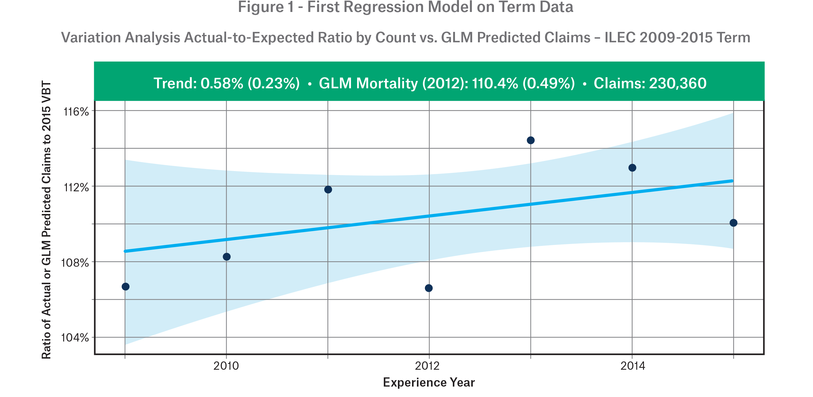
To start, the algorithm fits the regression model to the specified data. The result is illustrated in Figure 1. Mean trend is borderline significantly positive.

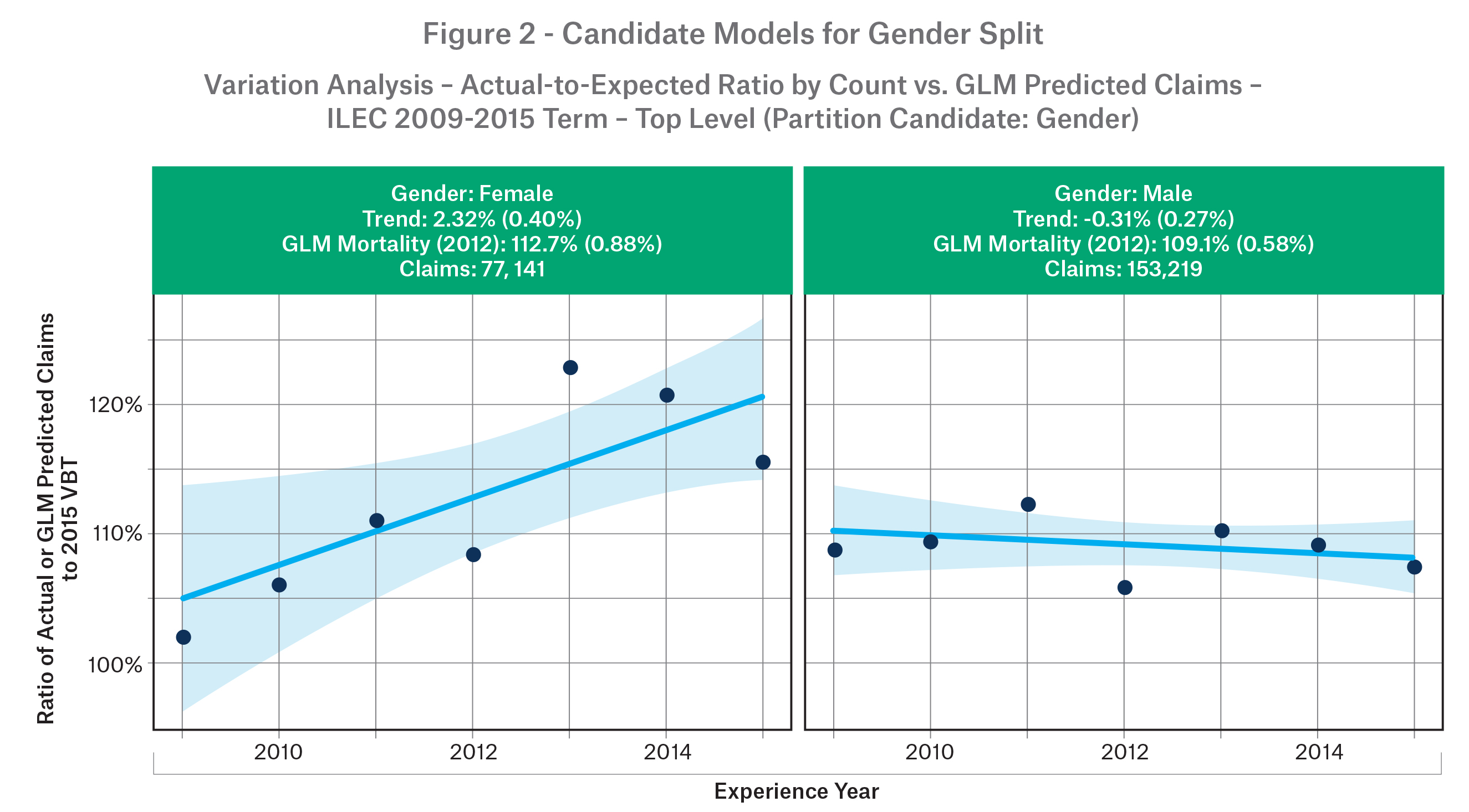
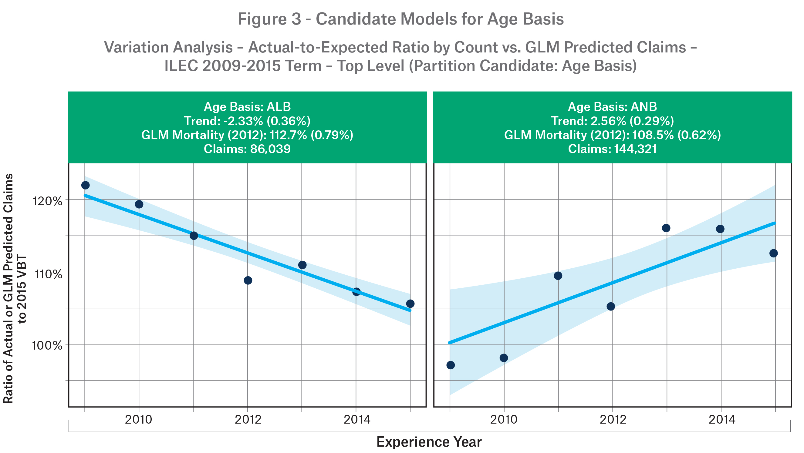
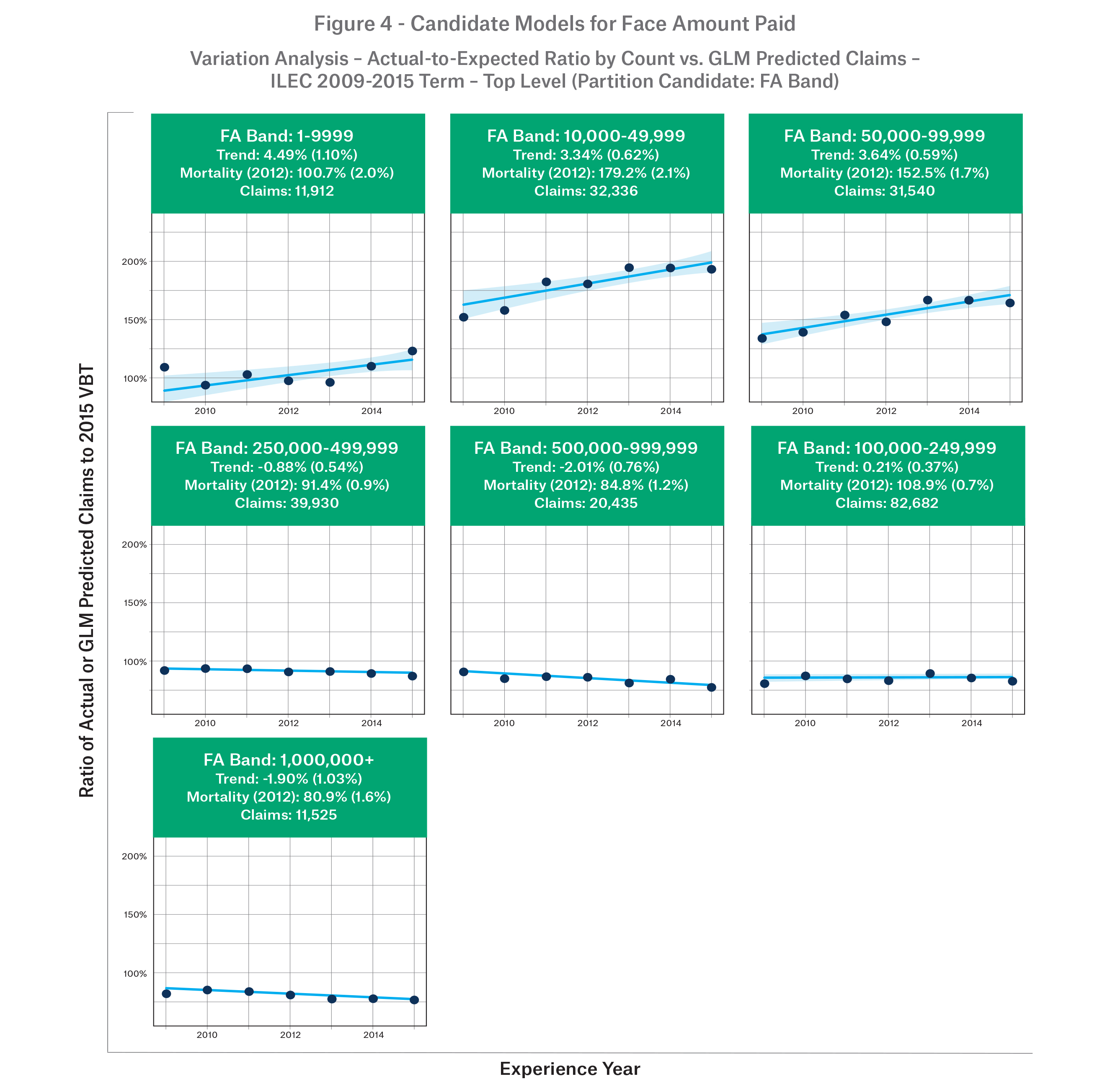
There are twelve variables to test. For this article, we demonstrate the first three and stop with face amount band, which was what was ultimately chosen at the top level. The first variable to test in the list is gender. In Figure 2, we see the models for a potential split. While there is a lot of unmodeled trend variation for females, there is less so for males. Moreover, the mean mortality level has small variation. The second is age basis. In Figure 3, This appears to be a promising split, with age nearest showing deterioration yet small variation for mean mortality. 

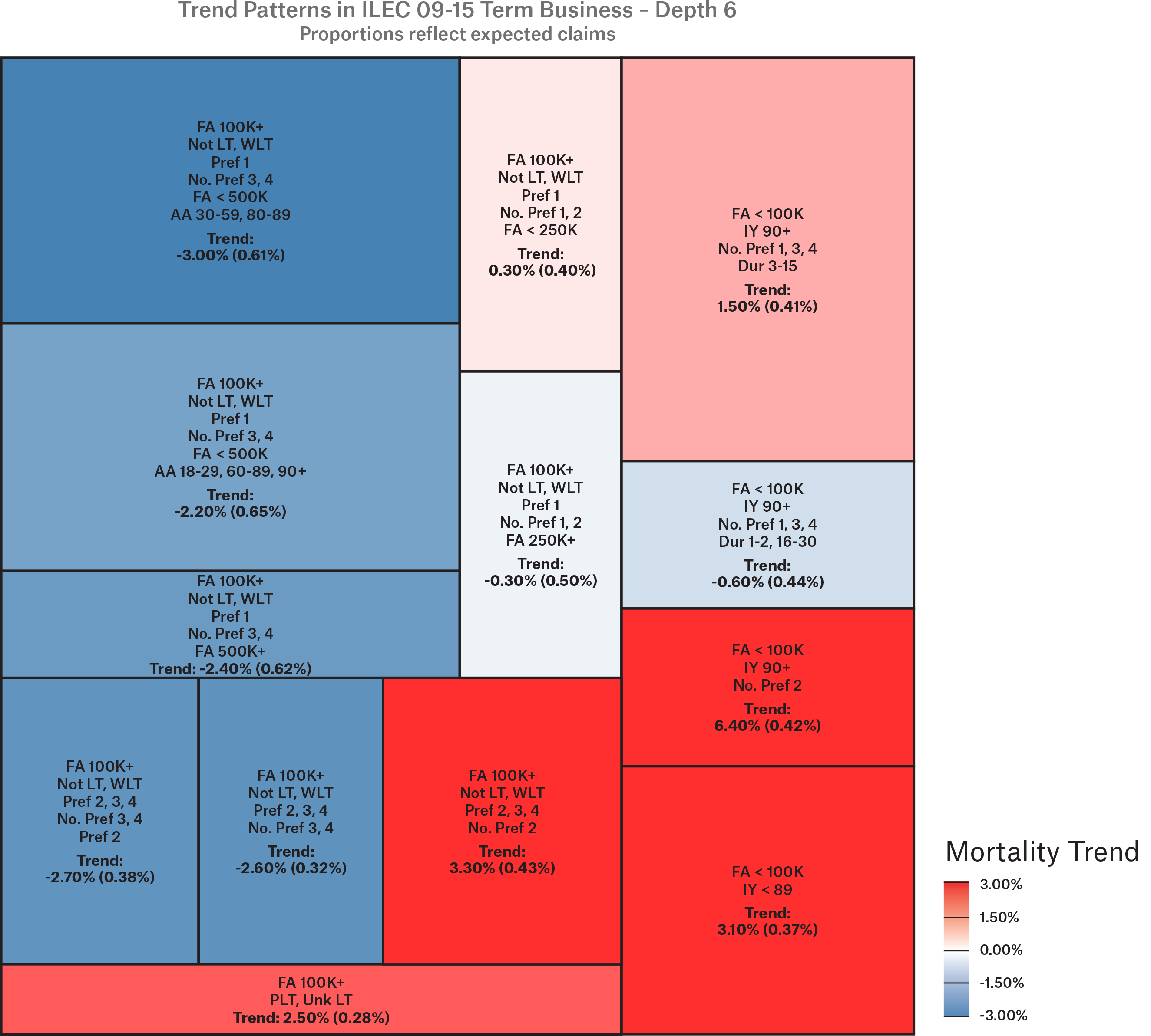
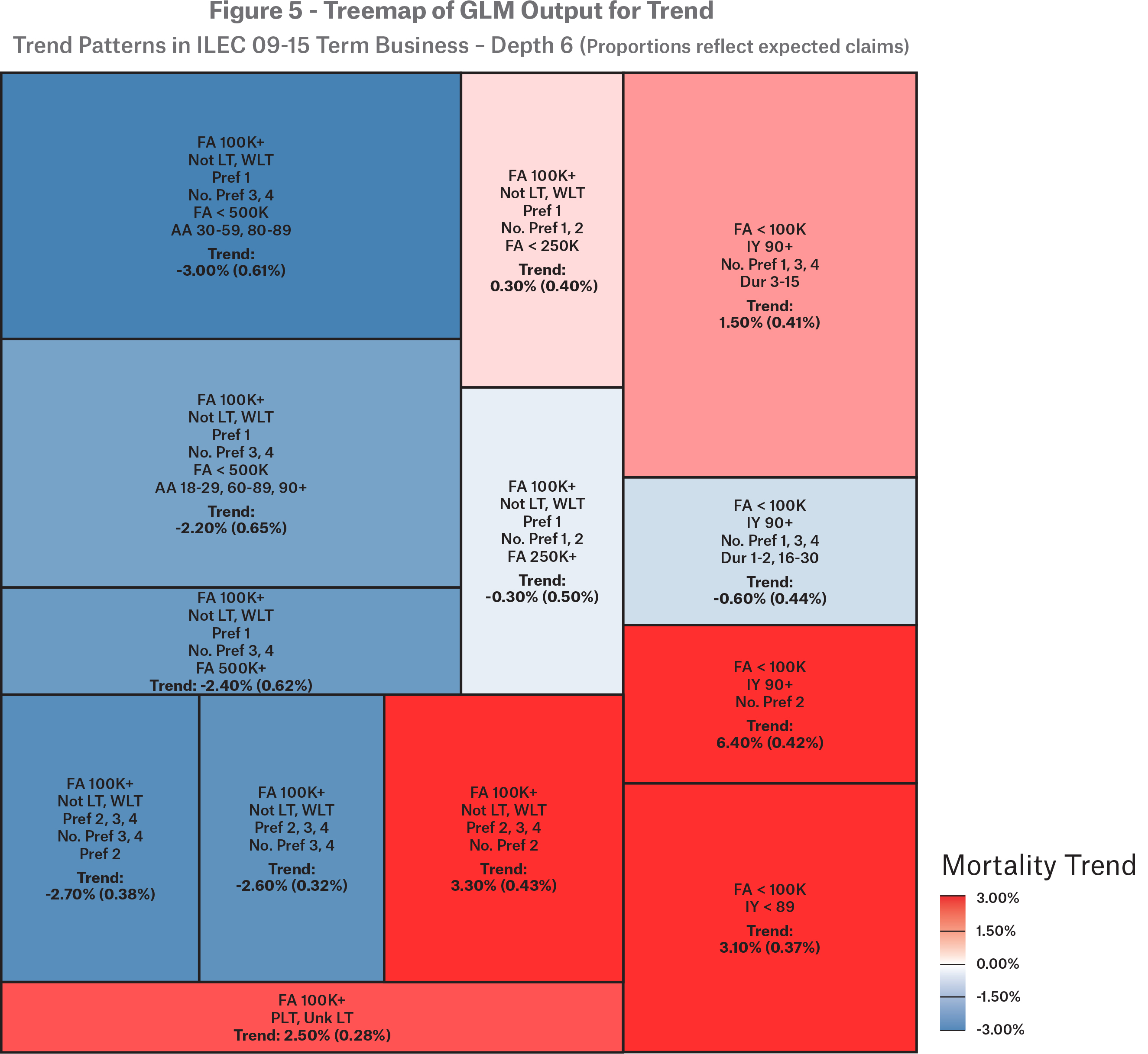
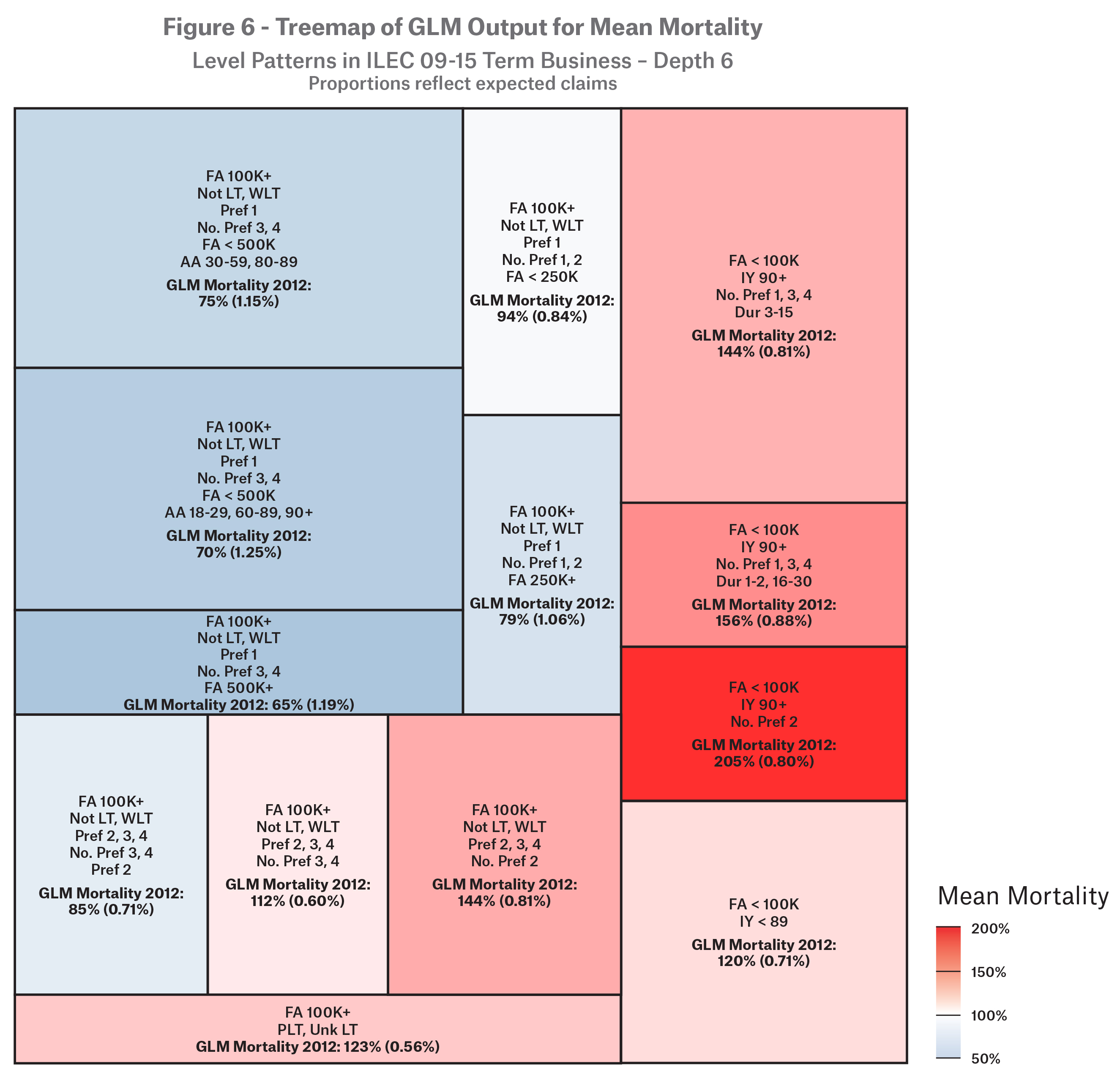
The algorithm continues and builds a tree recursively defined by split conditions with a GLM at each node and leaf of the tree. By default, the partykit package expresses the results as a traditional tree, either in text or plot form. To get around the limitations of the default output, I expressed the results as a treemap as in Figure 5. Note that the minimum node size was 10,000 expected claims, so each block carries no less than that.

If you let your eyes wander, some findings emerge:

1. Face amounts less than 100,000 exhibited deterioration (the right third of the square). In the instance of 2-class preferred systems, deterioration was torrid at 6.4% (SE 0.42%) on average per year. One possible exception was the light blue block, but this is statistically not significant (SE 0.44%).

2. Face amounts 100,000 and higher witnessed improvement in general, with two exceptions.

• The lower left corner contains post-level term and unknown level term business. The trend here is potentially contaminated with slope misalignment between the experience and base table. The net deterioration is 2.5% (SE 0.28%) per year on average.
• The angry red block above it is residual standard of 2-class preferred systems including the non-level term and within level term business. Note that within level term dominates the block. There was substantial deterioration of 3.3% on average per year (SE 0.43%).

3. Right next to the angry red block is a very blue block which contains residual standard of 3- and 4-class preferred systems. For these lives, there was substantial improvement on average of 2.6% per year (SE 0.32%), partly offsetting the deterioration in the 2-class system.

What About Permanent Products? What About Analysis by Amount?

Permanent products have been omitted from this paper for brevity. The claim count is nearly 10x as large as for term products, with much longer issue year horizons and more insurance plan types.

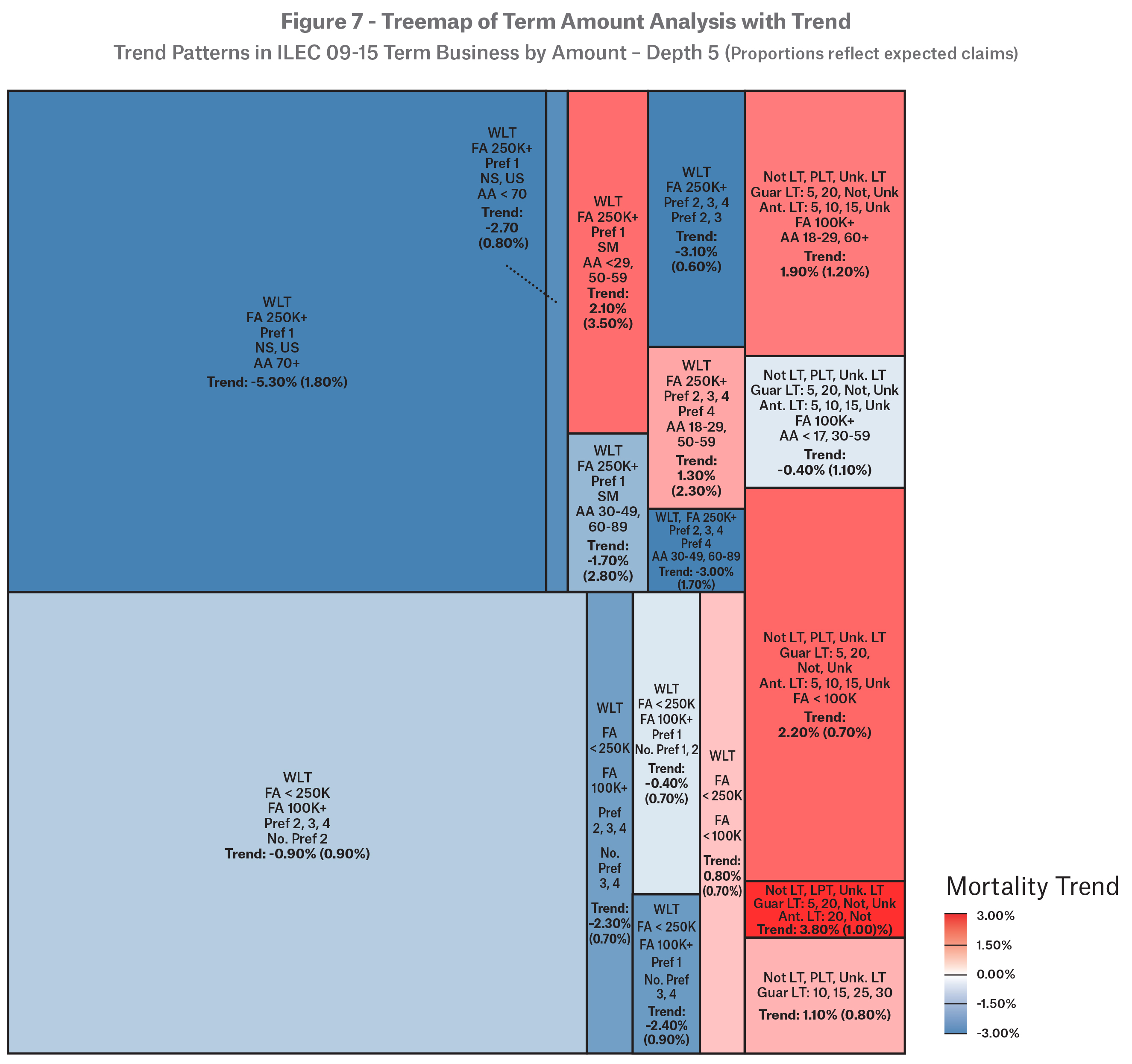
The analysis by amount for term products has a few differences. In terms of parameters, the GLM family is changed to a Tweedie distribution with parameter 1.2. The minimum size depends on the specified weighting vector. To encourage credible leaves, the minimum size is arbitrarily set to 10,000 * $50,000, or $500,000,000, and the maximum depth tree depth is set to 6. All but one of the resulting leaves has at least 10,000 actual claims.

The term amount analysis led to a different tree. The first split was within level term versus not within level term. Further splits within level term were along face amount, preferred class, smoker/non-smoker, and attained age. For other than within level term, splits occurred along term length, face amount, and attained age lines. The final tree map is in Figure 7.

Limitations

The intent of the analysis was to unravel some of the riddles around trend in the ILEC 2009-2015 dataset. Since the minimum claim size per node was so large, it is likely that more insights can be gained by allowing the algorithm to drill deeper or changing the GLM model template used for each node.

I encountered a few problems when applying the glmtree function in the partykit package to the data. The first was data sparsity with depth; that is, there must be enough diversity in the data to support fitting a GLM within any proposed node. An early attempt at GLM trees was to have the GLM model template be an interaction between attained
age group and duration group. The result would be an optimal subdivision of the data with a custom select-and-ultimate mortality table for each node of the tree. However, not every combination of age and duration will be available in every subset, or there may be exposures but no claims for a row.

The second was weighting. By default, the glmtree function applies the same weights parameter to both the GLM fitting and the parameter fluctuation tests. While this is fine for most applications, it is not when using an offset in a Poisson model. If a weights vector is specified, the resulting GLMs will be skewed. If no weight is specified, the individual GLMs are fine, but the parameter fluctuation tests will weight equally each row of the data. Thus, it was necessary to customize the code to allow separate weights for the GLM fitting steps.

The third was lack of accommodation for splines. I had attempted to build a “gamtree” function where the models within each node were GAMs. Adapting the spline parameters to parameter fluctuation tests proved challenging, and I ultimately set the task aside for later research.

Future Directions

GLM trees are a valuable tool that help to bridge the gap between the needs of traditional actuarial analysis and the potential of modern data science methods. As an exploratory tool, it can illuminate interesting structures in datasets. Using the typical recipe with training and test data, it can be applied as a predictive model. It can also be a point of departure for additional analysis, such as exposing where to focus further analysis or as a starting point for more sophisticated and targeted models.